Finding Least Cost Paths

Finding Least Cost Paths

Many applications need to find least cost paths through weighted directed graphs. The problem is to find a path through a graph in which non-negative weights are associated with the arcs. We will use Dijkstra's algorithm to determine the path.

This will be an opportunity to use several previously introduced libraries. In the order of appearance, the following modules will be used: Genlex and Printf for input and output, the module Weak to implement a cache, the module Sys to track the time saved by a cache, and the Awi library to construct a graphical user interface. The module Sys is also used to construct a standalone application that takes the name of a file describing the graph as a command line argument.

Graph Representions

A weighted directed graph is defined by a set of nodes, a set of edges, and a mapping from the set of edges to a set of values. There are numerous implementations of the data type weighted directed graph.

adjacency matrices:
each element (m(i,j)) of the matrix represents an edge from node i to j and the value of the element is the weight of the edge;
adjacency lists:
each node i is associated with a list [(j₁,w₁); ..; (j_n,w_n)] of nodes and each triple (i, j_k, w_k) is an edge of the graph, with weight w_k;
a triple:
a list of nodes, a list of edges and a function that computes the weights of the edges.

The behavior of the representations depends on the size and the number of edges in the graph. Since one goal of this application is to show how to cache certain previously executed computations without using all of memory, an adjacency matrix is used to represent weighted directed graphs. In this way, memory usage will not be increased by list manipulations.


# type  cost  = Nan | Cost of float;;
# type  adj_mat =  cost array array;;
# type 'a graph = { mutable ind : int; 
                    size : int; 
                    nodes : 'a array;  
                    m : adj_mat};;

The field size indicates the maximal number of nodes, the field ind the actual number of nodes.

We define functions to let us create graphs edge by edge.

The function to create a graph takes as arguments a node and the maximal number of nodes.


# let create_graph n s = 
   { ind = 0; size = s; nodes = Array.create s n; 
     m = Array.create_matrix s s Nan } ;;
val create_graph : 'a -> int -> 'a graph = <fun>

The function belongs_to checks if the node n is contained in the graph g.


# let belongs_to n g = 
   let rec aux i =
     (i < g.size) & ((g.nodes.(i) = n) or (aux (i+1)))
   in aux 0;;
val belongs_to : 'a -> 'a graph -> bool = <fun>

The function index returns the index of the node n in the graph g. If the node does not exist, a Not_found exception is thrown.


# let index n g = 
   let rec aux i = 
     if i >= g.size then raise Not_found
     else if g.nodes.(i) = n then i 
          else aux (i+1)
   in aux 0 ;;
val index : 'a -> 'a graph -> int = <fun>

The next two functions are for adding nodes and edges of cost c to graphs.


# let add_node n g = 
   if g.ind = g.size then failwith "the graph is full"
   else if belongs_to n g then failwith "the node already exists"
   else (g.nodes.(g.ind) <- n; g.ind <- g.ind + 1) ;;
val add_node : 'a -> 'a graph -> unit = <fun>
# let add_edge e1 e2 c g = 
   try
     let x = index e1 g and y = index e2 g in 
       g.m.(x).(y) <- Cost c 
   with Not_found -> failwith "node does not exist" ;;
val add_edge : 'a -> 'a -> float -> 'a graph -> unit = <fun>

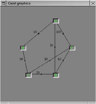
Now it is easy to create a complete weighted directed graph starting with a list of nodes and edges. The function test_aho constructs the graph of figure 13.8:


# let test_aho () = 
   let g = create_graph "nothing" 5 in 
     List.iter (fun x -> add_node x g) ["A"; "B"; "C"; "D"; "E"];
     List.iter (fun (a,b,c) -> add_edge a b c g) 
       ["A","B",10.;
        "A","D",30.;
        "A","E",100.0;
        "B","C",50.;
        "C","E",10.;
        "D","C",20.;
        "D","E",60.];
     for i=0 to g.ind -1 do g.m.(i).(i) <- Cost 0.0 done;
      g;;
val test_aho : unit -> string graph = <fun>
# let a = test_aho();;
val a : string graph =
  {ind=5; size=5; nodes=[|"A"; "B"; "C"; "D"; "E"|];
   m=[|[|Cost 0; Cost 10; Nan; Cost 30; Cost ...|]; ...|]}

Figure 13.8: The test graph

Constructing Graphs

It is tedious to directly construct graphs in a program. To avoid this, we define a concise textual representation for graphs. We can define the graphs in text files and construct them in applications by reading the text files.

The textual representation for a graph consists of lines of the following forms:

the number of nodes: SIZE number;
the name of a node: NODE name;
the cost of an edge: EDGE name1 name2 cost;
a comment: # comment.

For example, the following file, aho.dat, describes the graph of figure 13.8 :

SIZE 5
NODE A
NODE B
NODE C
NODE D
NODE E
EDGE A B 10.0
EDGE A D 30.0
EDGE A E 100.0
EDGE B C 50.
EDGE C E 10.
EDGE D C 20.
EDGE D E 60.

To read graph files, we use the lexical analysis module Genlex. The lexical analyser is constructed from a list of keywords keywords.

The function parse_line executes the actions associated to the key words by modifying the reference to a graph.


# let keywords = [ "SIZE"; "NODE"; "EDGE"; "#"];;
val keywords : string list = ["SIZE"; "NODE"; "EDGE"; "#"]
# let lex_line l = Genlex.make_lexer keywords (Stream.of_string l);;
val lex_line : string -> Genlex.token Stream.t = <fun>
# let parse_line g s = match  s with parser
   [< '(Genlex.Kwd  "SIZE"); '(Genlex.Int n) >] -> 
       g := create_graph "" n
 | [< '(Genlex.Kwd  "NODE"); '(Genlex.Ident name) >] -> 
       add_node name !g
 | [< '(Genlex.Kwd  "EDGE"); '(Genlex.Ident e1); 
      '(Genlex.Ident  e2); '(Genlex.Float c) >] -> 
       add_edge e1 e2 c !g
 | [< '(Genlex.Kwd  "#") >] -> ()
 | [<>] -> () ;;
val parse_line : string graph ref -> Genlex.token Stream.t -> unit = <fun>

The analyzer is used to define the function creating a graph from the description in the file:


# let create_graph name = 
   let g = ref {ind=0; size=0; nodes =[||]; m = [||]} in 
   let ic = open_in name in 
    try 
      print_string ("Loading "^name^": ");
      while true do 
       print_string "."; 
        let l = input_line ic in parse_line g (lex_line l)  
      done;
      !g
    with End_of_file -> print_newline(); close_in ic; !g ;;
val create_graph : string -> string graph = <fun>

The following command constructs a graph from the file aho.dat.


# let b = create_graph "PROGRAMMES/aho.dat" ;;
Loading PROGRAMMES/aho.dat: ..............
val b : string graph =
  {ind=5; size=5; nodes=[|"A"; "B"; "C"; "D"; "E"|];
   m=[|[|Nan; Cost 10; Nan; Cost 30; Cost 100|]; ...|]}

Dijkstra's Algorithm

Dijkstra's algorithm finds a least cost path between two nodes. The cost of a path between node n1 and node n2 is the sum of the costs of the edges on that path. The algorithm requires that costs always be positive, so there is no benefit in passing through a node more than once.

Dijkstra's algorithm effectively computes the minimal cost paths of all nodes of the graph which can be reached from a source node n1. The idea is to consider a set containing only nodes of which the least cost path to n1 is already known. This set is enlarged successively, considering nodes which can be accessed directly by an edge from one of the nodes already contained in the set. From these candidates, the one with the best cost path to the source node is added to the set.

To keep track of the state of the computation, the type comp_state is defined, as well as a function for creating an initial state:


# type comp_state = { paths : int array;
                     already_treated : bool array;
                     distances : cost array;
                     source : int; 
                     nn : int};;
# let create_state () =  { paths = [||]; already_treated = [||]; distances = [||]; 
                        nn = 0; source = 0};;

The field source contains the start node. The field already_treated indicates the nodes whose optimal path from the source is already known. The field nn indicates the total number of the graph's nodes. The vector distances holds the minimal distances between the source and the other nodes. For each node, the vector path contains the preceding node on the least cost path. The path to the source can be reconstructed from each node by using path.

Cost Functions

Four functions on costs are defined: a_cost to test for the existence of an edge, float_of_cost to return the floating point value, add_cost to add two costs and less_cost to check if one cost is smaller than another.


# let a_cost c = match c with Nan -> false | _-> true;;
val a_cost : cost -> bool = <fun>
# let float_of_cost c = match c with 
   Nan -> failwith "float_of_cost"
 | Cost x -> x;;
val float_of_cost : cost -> float = <fun>
# let add_cost  c1 c2 = match (c1,c2) with 
   Cost x, Cost y -> Cost (x+.y)
 | Nan, Cost y -> c2
 | Cost x, Nan -> c1 
 | Nan, Nan ->  c1;;
val add_cost : cost -> cost -> cost = <fun>
# let less_cost  c1 c2 = match (c1,c2) with 
   Cost x, Cost y -> x < y
 | Cost x, Nan -> true
 | _, _ ->  false;;
val less_cost : cost -> cost -> bool = <fun>

The value Nan plays a special role in the computations and in the comparison. We will come back to this when we have presented the main function (page ??).

Implementing the Algorithm

The search for the next node with known least cost path is divided into two functions. The first, first_not_treated, selects the first node not already contained in the set of nodes with known least cost paths. This node serves as the initial value for the second function, least_not_treated, which returns a node not already in the set with a best cost path to the source. This path will be added to the set.


# exception Found of int;;
exception Found of int
# let first_not_treated cs = 
   try 
     for i=0 to cs.nn-1 do 
       if not cs.already_treated.(i) then raise (Found i)
     done;
     raise Not_found;
     0
   with Found i -> i ;;
val first_not_treated : comp_state -> int = <fun>
# let least_not_treated p cs =
   let ni = ref p  
   and nd = ref cs.distances.(p) in 
     for i=p+1 to cs.nn-1 do 
       if not cs.already_treated.(i) then 
        if less_cost cs.distances.(i)  !nd then 
          ( nd := cs.distances.(i);
            ni := i )
     done;
     !ni,!nd;;
val least_not_treated : int -> comp_state -> int * cost = <fun>

The function one_round selects a new node, adds it to the set of treated nodes and computes the distances for any next candidates.


# exception No_way;;
exception No_way
# let one_round cs  g = 
   let p = first_not_treated cs  in 
   let np,nc = least_not_treated p cs in
     if not(a_cost nc  ) then raise No_way 
     else 
     begin
       cs.already_treated.(np) <- true;
       for i = 0 to cs.nn -1 do
         if not cs.already_treated.(i) then 
         if a_cost g.m.(np).(i) then
           let ic = add_cost cs.distances.(np)  g.m.(np).(i) in 
             if less_cost ic cs.distances.(i)   then (
               cs.paths.(i) <- np;
               cs.distances.(i) <- ic
              ) 
       done;
       cs
     end;;
val one_round : comp_state -> 'a graph -> comp_state = <fun>

The only thing left in the implementation of Dijkstra's algorithm is to iterate the preceding function. The function dij takes a node and a graph as arguments and returns a value of type comp_state, with the information from which the least cost paths from the source to all the reachable nodes of the graph can be deduced.


# let dij s g = 
   if belongs_to s g then 
   begin
     let i = index s g in 
     let cs = { paths = Array.create g.ind (-1) ;
                already_treated = Array.create g.ind false;
                distances = Array.create g.ind Nan;
                nn = g.ind;
                source = i}  in
       cs.already_treated.(i) <- true; 
       for j=0 to g.ind-1 do 
         let c = g.m.(i).(j) in 
           cs.distances.(j) <- c;
           if a_cost c then cs.paths.(j) <- i 
       done;
       try
         for k = 0 to cs.nn-2 do 
           ignore(one_round cs g) 
         done;
         cs
       with No_way -> cs
   end
   else failwith "dij: node unknown";;
val dij : 'a -> 'a graph -> comp_state = <fun>

Nan is the initial value of the distances. It represents an infinite distance, which conforms to the comparison function less_cost. In contrast, for the addition of costs (function add_cost), this value is treated as a zero. This allows a simple implementation of the table of distances.

Now the search with Dijkstra's algorithm can be tested.


# let g = test_aho ();;
# let r = dij "A" g;;

The return values are:


# r.paths;;
- : int array = [|0; 0; 3; 0; 2|]
# r.distances;;
- : cost array = [|Cost 0; Cost 10; Cost 50; Cost 30; Cost 60|]

Displaying the Results

To make the results more readable, we now define a display function.

The table paths of the state returned by dij only contains the last edges of the computed paths. In order to get the entire paths, it is necessary to recursively go back to the source.


# let display_state f (g,st)  dest = 
   if belongs_to dest g then 
      let d = index dest g in
        let rec aux is = 
           if is = st.source then Printf.printf "%a"  f g.nodes.(is)
           else (
             let old = st.paths.(is) in 
             aux old;
             Printf.printf " -> (%4.1f) %a" (float_of_cost g.m.(old).(is))
                                          f g.nodes.(is)  
           )
        in 
          if not(a_cost st.distances.(d)) then Printf.printf "no way\n"
          else (
            aux d;
            Printf.printf " = %4.1f\n" (float_of_cost st.distances.(d)));;
val display_state :
  (out_channel -> 'a -> unit) -> 'a graph * comp_state -> 'a -> unit = <fun>

This recursive function uses the command stack to display the nodes in the right order. Note that the use of the format "a" requires the function parameter f to preserve the polymorphism of the graphs for the display.

The optimal path between the nodes "A" (index 0) and "E" (index 4) is displayed in the following way:


# display_state (fun x y -> Printf.printf "%s!" y) (a,r) "E";;
A! -> (30.0) D! -> (20.0) C! -> (10.0) E! = 60.0
- : unit = ()

The different nodes of the path and the costs of each route are shown.

Introducing a Cache

Dijkstra's algorithm computes all least cost paths starting from a source. The idea of preserving these least cost paths for the next inquiry with the same source suggests itself. However, this storage could occupy a considerable amount of memory. This suggests the use of ``weak pointers.'' If the results of a computation starting from a source are stored in a table of weak pointers, it will be possible for the next computation to check if the computation has already been done. Because the pointers are weak, the memory occupied by the states can be freed by the garbage collector if needed. This avoids interrupting the rest of the program through the allocation of too much memory. In the worst case, the computation has to be repeated for a future inquiry.

Implementing a Cache

A new type 'a comp_graph is defined:


# type 'a comp_graph =  
   { g : 'a graph; w : comp_state Weak.t } ;;

The fields g and w correspond to the graph and to the table of weak pointers, pointing to the computation states for each possible source.

Such values are constructed by the function create_comp_graph.


# let create_comp_graph g = 
   { g = g;
     w = Weak.create g.ind } ;;
val create_comp_graph : 'a graph -> 'a comp_graph = <fun>

The function dij_quick checks to see if the computation has already been done. If it has, the stored result is returned. Otherwise, the computation is executed and the result is registered in the table of weak pointers.


# let dij_quick s cg = 
   let i = index s cg.g in 
     match Weak.get cg.w i with 
       None -> let cs = dij s cg.g in 
                 Weak.set cg.w i (Some cs);
                 cs
     | Some cs -> cs;;
val dij_quick : 'a -> 'a comp_graph -> comp_state = <fun>

The display function still can be used:


# let cg_a = create_comp_graph a in
 let r = dij_quick "A" cg_a in
  display_state (fun x y -> Printf.printf "%s!" y) (a,r) "E" ;;
A! -> (30.0) D! -> (20.0) C! -> (10.0) E! = 60.0
- : unit = ()

Performance Evaluation

We will test the performance of the functions dij and dij_quick by iterating each one on a random list of sources. In this way an application which frequently computes least cost paths is simulated (for example a railway route planning system).

We define the following function to time the calculations:


# let exe_time f g ss =
   let t0 = Sys.time() in
    Printf.printf "Start (%5.2f)\n" t0;
    List.iter (fun s -> ignore(f s g)) ss;
    let t1 = Sys.time() in
     Printf.printf "End (%5.2f)\n" t1;
     Printf.printf "Duration = (%5.2f)\n" (t1 -. t0) ;;
val exe_time : ('a -> 'b -> 'c) -> 'b -> 'a list -> unit = <fun>

We create a random list of 20000 nodes and measure the performance on the graph a:


# let ss = 
  let ss0 = ref [] in
  let i0 = int_of_char 'A' in
  let new_s i = Char.escaped (char_of_int (i0+i)) in
  for i=0 to 20000 do ss0 := (new_s (Random.int a.size))::!ss0 done;
  !ss0 ;;
val ss : string list =
  ["A"; "B"; "D"; "A"; "E"; "C"; "B"; "B"; "D"; "E"; "B"; "E"; "C"; "E"; "E";
   "D"; "D"; "A"; "E"; ...]
# Printf.printf"Function dij :\n";
 exe_time dij a ss ;;
Function dij :
Start ( 1.14)
End ( 1.46)
Duration = ( 0.32)
- : unit = ()
# Printf.printf"Function dij_quick :\n";
 exe_time dij_quick (create_comp_graph a) ss ;;
Function dij_quick :
Start ( 1.46)
End ( 1.50)
Duration = ( 0.04)
- : unit = ()

The results confirm our assumption. The direct access to a result held in the cache is considerably faster than a second computation of the result.

A Graphical Interface

We use the Awi library to construct a graphical interface to display graphs. The interface allows selection of the source and destination nodes of the path. When the path is found, it is displayed graphically. We define the type 'a gg, containing fields describing the graph and the computation, as well as fields of the graphical interface.


#  #load "PROGRAMMES/awi.cmo";;


# type 'a gg = { mutable src : 'a * Awi.component; 
                mutable dest : 'a * Awi.component;
                pos : (int * int) array;
                cg : 'a comp_graph;
                mutable state : comp_state;
                mutable main : Awi.component;
                to_string : 'a -> string;
                from_string : string -> 'a } ;;

The fields src and dest are tuples (node, component), associating a node and a component. The field pos contains the position of each component. The field main is the main container of the set of components. The two functions to_string and from_string are conversion functions between type 'a and strings. The elements necessary to construct these values are the graph information, the position table and the conversion functions.


# let create_gg cg vpos ts fs = 
   {src = cg.g.nodes.(0),Awi.empty_component;
    dest = cg.g.nodes.(0),Awi.empty_component;
    pos = vpos;
    cg = cg;
    state = create_state () ;
    main = Awi.empty_component;
    to_string = ts;
    from_string = fs};;
val create_gg :
  'a comp_graph ->
  (int * int) array -> ('a -> string) -> (string -> 'a) -> 'a gg = <fun>

Visualisation

In order to display the graph, the nodes have to be drawn, and the edges have to be traced. The nodes are represented by button components of the Awi library. The edges are traced directly in the main window. The function display_edge displays the edges. The function display_shortest_path displays the found path in a different color.

Drawing Edges

An edge connects two nodes and has an associated weight. The connection between two nodes can be represented by a line. The main difficulty is indicating the orientation of the line. We choose to represent it by an arrow. The arrow is rotated by the angle the line has with the abscissa (the x-axis) to give it the proper orientation. Finally, the costs are displayed beside the edge.

To draw the arrow of an edge we define the functions rotate and translate which care respectively for rotation and shifting. The function display_arrow draws the arrow.


# let rotate l a = 
   let ca = cos a  and sa = sin a in 
     List.map (function (x,y) -> ( x*.ca +. -.y*.sa, x*.sa +. y*.ca)) l;;
val rotate : (float * float) list -> float -> (float * float) list = <fun>
# let translate l (tx,ty) = 
   List.map (function (x,y) -> (x +. tx, y +. ty)) l;;
val translate :
  (float * float) list -> float * float -> (float * float) list = <fun>
# let display_arrow (mx,my) a = 
   let triangle = [(5.,0.); (-3.,3.); (1.,0.); (-3.,-3.); (5.,0.)] in
   let tr =  rotate triangle a in 
   let ttr = translate tr (mx,my) in 
   let tt = List.map (function (x,y) -> (int_of_float x, int_of_float y)) ttr 
   in
     Graphics.fill_poly (Array.of_list tt);;
val display_arrow : float * float -> float -> unit = <fun>

The position of the text indicating the weight of an edge depends on the angle of the edge.


# let display_label (mx,my) a lab = 
   let (sx,sy) = Graphics.text_size lab in
   let pos = [ float(-sx/2),float(-sy) ] in 
   let pr = rotate pos a in
   let pt = translate pr (mx,my) in 
     let px,py = List.hd pt in 
       let ox,oy = Graphics.current_point () in 
         Graphics.moveto ((int_of_float mx)-sx-6) 
                          ((int_of_float my) );
         Graphics.draw_string lab;
         Graphics.moveto ox oy;;
val display_label : float * float -> float -> string -> unit = <fun>

The preceding functions are now used by the function display_edge. Parameters are the graphical interface gg, the nodes i and j, and the color (col) to use.


# let display_edge gg col i j = 
   let g = gg.cg.g in  
   let x,y = gg.main.Awi.x,gg.main.Awi.y in 
     if a_cost g.m.(i).(j) then (
       let (a1,b1) = gg.pos.(i)
       and (a2,b2) = gg.pos.(j) in 
         let x0,y0 = x+a1,y+b1   and x1,y1 = x+a2,y+b2 in
         let rxm =  (float(x1-x0)) /. 2.  and rym =  (float(y1-y0)) /. 2. in
         let xm = (float x0) +. rxm and ym = (float y0) +. rym in
           Graphics.set_color col;
           Graphics.moveto x0 y0;
           Graphics.lineto x1 y1;
           let a =  atan2 rym rxm in 
           display_arrow (xm,ym) a;
           display_label (xm,ym) a 
             (string_of_float(float_of_cost g.m.(i).(j))));;
val display_edge : 'a gg -> Graphics.color -> int -> int -> unit = <fun>

Displaying a Path

To display a path, all edges along the path are displayed. The graphical display of a path towards a destination uses the same technique as the textual display.


# let rec display_shortest_path gg col dest = 
   let g = gg.cg.g in 
     if belongs_to dest g then 
       let d = index dest g in
        let rec aux is = 
           if is = gg.state.source then ()
           else (
             let old = gg.state.paths.(is) in 
               display_edge gg col old is;
               aux old )
        in 
          if not(a_cost gg.state.distances.(d)) then Printf.printf "no way\n"
          else aux d;;
val display_shortest_path : 'a gg -> Graphics.color -> 'a -> unit = <fun>

Displaying a Graph

The function display_gg displays a complete graph. If the destination node is not empty, the path between the source and the destination is traced.


#  let display_gg gg () =  
   Awi.display_rect gg.main ();
   for i=0 to gg.cg.g.ind -1 do 
     for j=0 to gg.cg.g.ind -1 do 
       if i<> j then display_edge gg (Graphics.black) i j 
     done
   done;
   if snd gg.dest != Awi.empty_component then 
      display_shortest_path gg Graphics.red (fst gg.dest);;
val display_gg : 'a gg -> unit -> unit = <fun>

The Node Component

The nodes still need to be drawn. Since the user is allowed to choose the source and destination nodes, we define a component for nodes.

The user's main action is choosing the end nodes of the path to be found. Thus a node must be a component that reacts to mouse clicks, using its state to indicate if it has been chosen as a source or destination. We choose the button component, which reacts to mouse clicks.

Node Actions

It is necessary to indicate node selection. To show this, the background color of a node is changed by the function inverse.


# let inverse b = 
   let gc = Awi.get_gc b in 
     let fcol = Awi.get_gc_fcol gc 
     and bcol = Awi.get_gc_bcol gc in 
       Awi.set_gc_bcol gc fcol;
       Awi.set_gc_fcol gc bcol;;
val inverse : Awi.component -> unit = <fun>

The function action_click effects this selection. It is called when a node is clicked on by the mouse. As parameters it takes the node associated with the button and the graph to modify the source or the destination of the search. When both nodes are selected, the function dij_quick finds a least cost path.

            
# let action_click node gg b bs = 
   let (s1,s) = gg.src
   and (s2,d) = gg.dest in 
    if  s == Awi.empty_component then (
      gg.src  <- (node,b); inverse b )
    else 
     if d == Awi.empty_component then ( 
       inverse b;
       gg.dest <- (node,b); 
       gg.state <- dij_quick s1 gg.cg;
      display_shortest_path gg (Graphics.red) node
     ) 
     else (inverse s; inverse d;
           gg.dest <- (s2,Awi.empty_component);
           gg.src <- node,b; inverse b);;
val action_click : 'a -> 'a gg -> Awi.component -> 'b -> unit = <fun>

Creating an Interface

The main function to create an interface takes an interface graph and a list of options, creates the different components and associates them with the graph. The parameters are the graph (gg), its dimensions (gw and gh), a list of graph and node options (lopt) and a list of node border options (lopt2).

  
# let main_gg gg gw gh lopt lopt2 = 
   let gc = Awi.make_default_context () in 
     Awi.set_gc gc lopt; 
 (* compute the maximal button size *)
     let vs = Array.map gg.to_string gg.cg.g.nodes in 
     let vsize = Array.map Graphics.text_size  vs in 
       let w = Array.fold_right (fun (x,y) -> max x)  vsize 0 
       and h = Array.fold_right (fun (x,y) -> max y)  vsize 0 in   
 (* create the main panel *)   
       gg.main <- Awi.create_panel true gw gh lopt;
       gg.main.Awi.display <- display_gg gg;
 (* create the buttons *)
         let vb_bs = 
           Array.map (fun x -> x,Awi.create_button (" "^(gg.to_string x)^" ") 
                        lopt)
                      gg.cg.g.nodes in 
           let f_act_b = Array.map (fun (x,(b,bs)) -> 
                                    let ac = action_click x  gg b
                                    in Awi.set_bs_action bs ac)  vb_bs in
           let bb = 
             Array.map (function (_,(b,_)) -> Awi.create_border b lopt2) vb_bs 
           in 
             Array.iteri 
               (fun i (b) -> let x,y = gg.pos.(i) in 
                               Awi.add_component gg.main  b 
                                 ["PosX",Awi.Iopt (x-w/2); 
                                  "PosY", Awi.Iopt (y-h/2)]) bb;
           ();;
val main_gg :
  'a gg ->
  int ->
  int -> (string * Awi.opt_val) list -> (string * Awi.opt_val) list -> unit =
  <fun>

The buttons are created automatically. They are positioned on the main window.

Testing the Interface

Everything is ready to create an interface now. We use a graph whose nodes are character strings to simplify the conversion functions. We construct the graph gg as follows:


# let id x = x;;
# let pos =  [| 200, 300; 80, 200 ; 100, 100; 200, 100;  260, 200 |];; 
# let gg = create_gg  (create_comp_graph (test_aho())) pos id id;;
# main_gg  gg 400 400 ["Background", Awi.Copt  (Graphics.rgb 130 130 130);
             "Foreground",Awi.Copt  Graphics.green] 
 [ "Relief", Awi.Sopt "Top";"Border_size", Awi.Iopt 2];;

Calling Awi.loop true false gg.main;; starts the interaction loop of the Awi library.

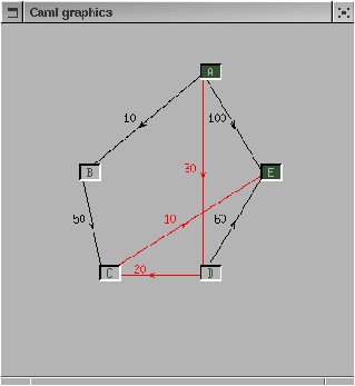
Figure 13.9: Selecting the nodes for a search

Figure 13.9 shows the computed path between the nodes "A" and "E". The edges on the path have changed their color.

Creating a Standalone Application

We will now show the steps needed to construct a standalone application. The application takes the name of a file describing the graph as an argument. For standalone applications, it is not necesary to have an Objective CAML distribution on the execution machine.

A Graph Description File

The file containes information about the graph as well as information used for the graphical interface. For the latter information, we define a second format. From this graphical description, we construct a value of the type g_info.


# type g_info = {npos : (int * int) array;
                mutable opt : Awi.lopt;
                mutable g_w : int;
                mutable g_h : int};;

The format for the graphical information is described by the four key words of list key2.


# let key2 = ["HEIGHT"; "LENGTH"; "POSITION"; "COLOR"];;
val key2 : string list = ["HEIGHT"; "LENGTH"; "POSITION"; "COLOR"]
# let lex2 l = Genlex.make_lexer key2 (Stream.of_string l);;
val lex2 : string -> Genlex.token Stream.t = <fun>

# let pars2 g gi s = match s with parser 
    [< '(Genlex.Kwd "HEIGHT"); '(Genlex.Int i) >] -> gi.g_h <- i
 |  [< '(Genlex.Kwd "LENGTH"); '(Genlex.Int i) >] -> gi.g_w <- i
 |  [< '(Genlex.Kwd "POSITION"); '(Genlex.Ident s);
       '(Genlex.Int i); '(Genlex.Int j) >] -> gi.npos.(index s g) <- (i,j)
 |  [< '(Genlex.Kwd "COLOR"); '(Genlex.Ident s);
       '(Genlex.Int r); '(Genlex.Int g); '(Genlex.Int b) >] ->
            gi.opt <- (s, Awi.Copt (Graphics.rgb r g b))::gi.opt
 | [<>] -> ();;
val pars2 : string graph -> g_info -> Genlex.token Stream.t -> unit = <fun>

Creating the Application

The function create_graph takes the name of a file as input and returns a couple composed of a graph and associated graphical information.


# let create_gg_graph name = 
   let g = create_graph name in 
     let gi = {npos = Array.create g.size (0,0); opt=[]; g_w =0; g_h = 0;} in
   let ic = open_in name in 
   try 
     print_string ("Loading (pass 2) " ^name ^" : ");
     while true do 
       print_string ".";
       let l = input_line ic in pars2 g gi (lex2 l)
     done ;
     g,gi
   with End_of_file -> print_newline(); close_in ic; g,gi;;
val create_gg_graph : string -> string graph * g_info = <fun>

The function create_app constructs the interface of a graph.


# let create_app name = 
   let g,gi = create_gg_graph name in
   let size = (string_of_int gi.g_w) ^ "x" ^ (string_of_int gi.g_h) in 
   Graphics.open_graph (" "^size);
   let gg = create_gg (create_comp_graph g) gi.npos id id in
   main_gg gg gi.g_w gi.g_h
     [ "Background", Awi.Copt (Graphics.rgb 130 130 130) ;
       "Foreground", Awi.Copt Graphics.green ]
     [ "Relief", Awi.Sopt "Top" ; "Border_size", Awi.Iopt 2 ] ;
   gg;;
val create_app : string -> string gg = <fun>

Finally, the function main takes the name of the file from the command line, constructs a graph with an interface and starts the interaction loop on the main component of the graph interface.


# let main () = 
   if (Array.length Sys.argv ) <> 2 
   then Printf.printf "Usage: dij.exe filename\n"
   else 
     let gg = create_app Sys.argv.(1) in 
       Awi.loop true false gg.main;;
val main : unit -> unit = <fun>

The last expression of that program starts the function main.

The Executable

The motivation for making a standalone application is to support its distribution. We collect the types and functions described in this section in the file dij.ml. Then we compile the file, adding the different libraries which are used. Here is the command to compile it under Linux.

ocamlc -custom -o dij.exe graphics.cma awi.cmo graphs.ml \
    -cclib -lgraphics -cclib -L/usr/X11/lib -cclib -lX11

Compiling standalone applications using the Graphics library is described in chapters 5 and 7.

Final Notes

The skeleton of this application is sufficiently general to be used in contexts other than the search for traveling paths. Different types of problems can be represented by a weighted graph. For example the search for a path in a labyrinth can be coded in a graph where each intersection is a node. Finding a solution corresponds to computing the shortest path between the start and the goal.

To compare the performance betwen C and Objective CAML, we wrote Dijkstra's algorithm in C. The C program uses the Objective CAML data structures to perform the calculations.

To improve the graphical interface, we add a textfield for the name of the file and two buttons to load and to store a graph. The user may then modify the positions of the nodes by mouse to improve the appearance.

A second improvement of the graphical interface is the ability to choose the form of the nodes. To display a button, a function tracing a rectangle is called. The display functions can be specialized to use polygons for nodes.